Overview

1. What led me to this project ?
   
2. Goals for this presentation
3. Problem Description
4. Data processing
5. EDA
6. Feature Buildings
7. Model Buildings
8. Comparing models
9. Conclusion
10. References

• Wanted to apply Big data method on the humanitarian sector and create an analytic value around one current issue.
• Found a rich dataset provided by Driven Data offering an open challenge until 2021 with data compiled from http://taarifa.org/ website and the Tanzanian Ministry of Water.
• Participate in an open - data challenge online.
  
• Build a data stand-alone project which responds to Project requirements and that makes first conclusions about predictions and highlights future improvements to be made to the scripts to improve model performance

• Present major steps required for project requirement
• Present you the framework I implemented to handle one online data challenge and receive advice if any to improve it !

• I had a little more time to prepare this presentation. I have used the package Slidify which is a tool to create, customize and publish, reproducible HTML5 slide decks using R Markdown.

• You can follow this slide within your browser by clicking to this link. I will ask you a small participation in a slide !

• The original goal is to predict whether a water pump is functional, functional but needs repairs or non functional based on a train dataset.

• This is an intermediate-level practice competition which allow us to train us to predict the operating condition of a water-point for each record in a dataset.

• A smart understanding of which water-points will fail can improve maintenance operations and ensure that clean, potable water is available to communities across Tanzania.

• Faced to an unsupervised classification problem

• The metric used for the competition is classification rate ( percentage of rows where the predicted class y in the submission matches the actual class y in the test set).

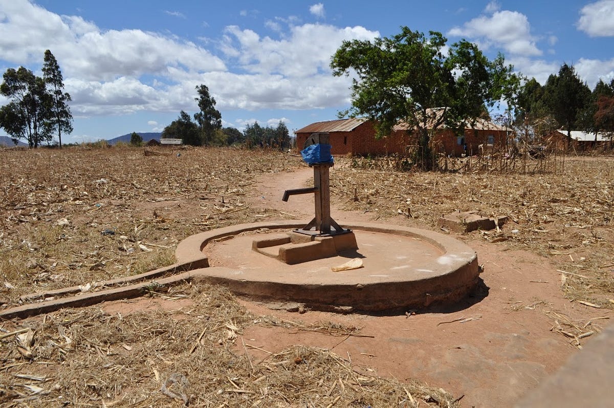
An example of a Water Pump - http://www.humanosphere.org/

• Get the data.
  • Usually, a data challenge provides a train and test datasets with test dataset target empty. Here the website, has separated train value and train labels ...

train_value <- read.csv("Trainingset_values.csv")
train_labels <-read.csv("Trainingset_label.csv")
test_values <- read.csv("Testset_value.csv")

• We merge the train value and the train label ...

train <- merge(train_labels, train_value)
test <- test_values

• and plot the first 6 rows of our train dataset.
  

• The labels in this dataset are simple. There are three possible values:

  Name	Description
  functional	the waterpoint is operational and there are no repairs needed
  functional needs repair	the waterpoint is operational, but needs repairs
  non functional	the waterpoint is not operational

• Let us describe the number of each pumps in status group and their proportions : Unbalanced dataset ?

       functional functional needs repair          non functional 
            32259                    4317                   22824 
  
       functional functional needs repair          non functional 
       0.54308081              0.07267677              0.38424242 
  

• Our dataset is pretty balanced but we can already notice that we have a great number of Missing values. We will see in future part how I managed it. First, let us do some EDA in order to better understand our data.

• Create 2 bar plots for quantity

• Create bar plot for quality_group

• Create bar plot for water point_type

• Create histogram for all variables

• Create a histogram for construction_year grouped by status_group

• Features building was maybe one of the most important part of my project.

• Very often in challenges, this part is a key part, allowing the models to really find performance. In order, we will address the following problems: reducing factor levels, handle missing and empty values.

• For feature engineering, it is better to combine training and the test sets together into one dataset. So I added a column subset in order to split the data later.

train$subset = "train"
test$subset = "test"
test$status_group<-""
data = rbind(train,test)

names(data)

• The data table contains an ID column, a subset indicator, a response column (status_group is functional, functional needs repair or non functional) and 38 features.

• Based on their names , we could conclude that some features have the same information but maybe at different levels (for example, extraction_type and extraction_type_group).

• For each grouping of features, we will keep both the coarser and the finer variables but group some of the smaller levels together so that categorical predictors have minimum levels.

• First, we will reduce factor levels if the number of a factor is small and thus irrelevant.This code shows us in descending order of n the frequency of each factor level and then we have the proportion.

data %>%
  group_by(extraction_type_class, extraction_type_group, extraction_type) %>% tally(sort=TRUE)
## # A tibble: 18 x 4
## # Groups:   extraction_type_class, extraction_type_group [13]
##    extraction_type_class extraction_type_group extraction_type               n
##    <fct>                 <fct>                 <fct>                     <int>
##  1 gravity               gravity               gravity                   33263
##  2 handpump              nira/tanira           nira/tanira               10205
##  3 other                 other                 other                      8102
##  4 submersible           submersible           submersible                5982
##  5 handpump              swn 80                swn 80                     4588
##  6 motorpump             mono                  mono                       3628
##  7 handpump              india mark ii         india mark ii              3029
##  8 handpump              afridev               afridev                    2208
##  9 submersible           submersible           ksb                        1790
## 10 rope pump             rope pump             other - rope pump           572
## 11 handpump              other handpump        other - swn 81              284
## 12 wind-powered          wind-powered          windmill                    152
## 13 handpump              india mark iii        india mark iii              135
## 14 motorpump             other motorpump       cemo                        108
## 15 handpump              other handpump        other - play pump           101
## 16 handpump              other handpump        walimi                       60
## 17 motorpump             other motorpump       climax                       41
## 18 handpump              other handpump        other - mkulima/shinyanga     2

prop.table((table(data$extraction_type_class)))
## 
##      gravity     handpump    motorpump        other    rope pump  submersible 
##  0.447986532  0.277602694  0.050868687  0.109117845  0.007703704  0.104673401 
## wind-powered 
##  0.002047138

We decide to class the small level to "other", meaning rope pump, wind-powered to other.

data$extraction_type_class[data$extraction_type_class=="rope pump"] <- "other"
data$extraction_type_class[data$extraction_type_class=="wind-powered"] <- "other"

We will remove middle level extraction_type_group and combine some of the smaller levels.

data = data %>%mutate(extraction_type = revalue(extraction_type,
                                     c("cemo" = "other motorpump",
                                       "climax" = "other motorpump",
                                       "other - mkulima/shinyanga" = "other handpump",
                                       "other - play pump" = "other handpump",
                                       "walimi" = "other handpump",
                                       "other - swn 81" = "swn",
                                       "swn 80" = "swn",
                                       "india mark ii" = "india mark",
                                       "india mark iii" = "india mark"))) %>%select( - extraction_type_group ) 

• I have done the same process for following variables : "quality_group", remove waterpoint_type_group., payment_type, Scheme_name, recorded by, ward variable and wpt-name, subvillage, lga.

• One difficulty in our dataset is that there is no clear missing values but only zeros. However, for some variables, it seems that having 0 in observation is not possible and can be seen as a missing value :
  funder, installer, gps_height, population, construction_year, and possibly, amount_tsh, latitude and longitude (given to the fact that Tanzania geographical position). We should re-code those variable to NA.

data = data %>%
  mutate(gps_height = ifelse(gps_height == 0, NA, gps_height)) %>%
  mutate(population = ifelse(population == 0, NA, population)) %>%
  mutate(amount_tsh = ifelse(amount_tsh == 0, NA, amount_tsh)) %>%
  mutate(longitude = ifelse(longitude == 0, NA, longitude)) %>%
  mutate(latitude = ifelse(latitude == 0, NA, latitude)) %>%
  mutate(construction_year = ifelse(construction_year == 0, NA, construction_year))

• Let us plot missing values distribution.
• We can observe that amount_tsh has a lot of NA and this variable is not very clear for the reader. We should remove it.

data = data %>% select( - amount_tsh)

• Then we have population and gps_height variables with more than 30 % of NA. Since these last variables contain important information, we should keep them.

• Since we will use Random Forest models, we have to re-code NA values to zeros.

data[is.na(data)] <- 0

We still have empty rows that we should resolve.

data$permit<- as.character(data$permit)
data$permit[data$permit==""]<-"unknown"
data$permit<-as.factor(data$permit)
data$scheme_management<- as.character(data$scheme_management)
data$scheme_management[data$scheme_management==""]<-"unknown"
data$scheme_management<-as.factor(data$scheme_management)
data$public_meeting<- as.character(data$public_meeting)
data$public_meeting[data$public_meeting==""]<-"unknown"
data$public_meeting<-as.factor(data$public_meeting)

• This ends our feature feature building part. I tried to take time for this part in our presentation as it important in data competition and in order to share methods.

• We are now ready to build our models !

First, we should unsplit data to build our final dataset and clean our environment for a peaceful mind.

trainset<-data[data$subset=="train",]
testset<-data[data$subset=="test",]
trainset<-trainset[-28]
testset<-testset[-28]

rm(train)
rm(test)
rm(test_values)
rm(train_labels)
rm(train_value)

When I applied my first models, it should be noted that I faced a factor and subseting problem. I found a solution by applying str and drop levels to our unsplit datasets.

str(data$status_group)
str(trainset$status_group)
str(trainset$status_group)

table(data$status_group)
table(trainset$status_group)
table(trainset$status_group)

trainset$status_group<-droplevels(trainset$status_group)
table(trainset$status_group)

• Random Forest reduces the variance of forecasts in a decision tree alone, thus improving performance. It does this by combining n decision trees in a bagging approach. We don't prune the tree. Each tree in the random forest is trained on a random subset of data. The predictions are then averaged.

• I have build model on the train dataset with following parameters :

• randomForest(status_group~.,data=trainset, ntree=300, do.trace=T)

• This graph comes from our first model and plot the importance of variable in our model.

• The second graph shows the evolution of error compared to the number of trees.

• We can apply our models on our testset and create our first submission file.

• We will see in our last part what were the results.

• In order to compare the models, we will build another Tree.

• Here we will use Boosted Tree aka XGBoost. XGBoost is a well-known and efficient open source implementation of the improved gradient tree algorithm.

• We are building a tree and looks which value is predicted poorly and assign to it higher weigh in our prediction.

• Let us build and predict our model with 1000 maximum number of boosting iterations with following parameters : xgboost::xgboost(data=data.matrix(trainset[,-2]),label=trainset[,2],nrounds=1000,params=list(booster="gbtree", eta=0.10, max_depth = 3, subsample = 0.50, colsample_bytree=0.50))

• Let's apply our model and create a second submission file.

I upload first submission of Random Forest to the Driven Data Platform

• For recall, Primary Evaluation Metric is Classification Rate \[ \frac{1}{N} \sum_{i=0}^N I(y_i = \hat{y_i}) \] It calculates the percentage of rows where the predicted class y^ in the submission matches the actual class, y in the test set. The maximum is 1 and the minimum is 0. The goal is to maximize the classification rate.
  

• Before we see finally our results, a quick quiz !

-Our second tree returned a better metric with 0.8179. This small increase has moved us up 15 places in the competition.

-So Boosted Tree was the best Tree model to predict whether a water pump is functional, functional but needs repairs or non functional.

-I decided to stop here as the 2 models gave almost the same results meaning that one should move again to feature building (any recommendation or ideas is welcome) so as to maximize Classification Rate.

-Thank you for your attention !

• Dr Jaroslaw Jozef Olejniczak- Big Data - SGH Spring 2020
  
• Community of Driven Data https://community.drivendata.org/c/pump-it-up-data-mining-the-water-table
• Stack Overflow community

photo from http://www.bookcovercafe.com/independent-publishing-q-and-a-series-01/